
Snowflake with Ray Air
Contents
Snowflake with Ray Air#
By using the Ray Snowflake connector to read and write data into and out of Ray Datasets, all of the capabilities of Ray AIR can be used to build end to end machine learning applications.
What is Ray AIR?#
Ray AI Runtime (AIR) is a scalable and unified toolkit for ML applications. AIR enables simple scaling of individual workloads, end-to-end workflows, and popular ecosystem frameworks, all in just Python.

AIR builds on Ray’s best-in-class libraries for Preprocessing, Training, Tuning, Scoring, Serving, and Reinforcement Learning to bring together an ecosystem of integrations.
ML Compute, Simplified#
Ray AIR aims to simplify the ecosystem of machine learning frameworks, platforms, and tools. It does this by leveraging Ray to provide a seamless, unified, and open experience for scalable ML:

Seamless Dev to Prod: AIR reduces friction going from development to production. With Ray and AIR, the same Python code scales seamlessly from a laptop to a large cluster.
Unified ML API: AIR’s unified ML API enables swapping between popular frameworks, such as XGBoost, PyTorch, and HuggingFace, with just a single class change in your code.
Open and Extensible: AIR and Ray are fully open-source and can run on any cluster, cloud, or Kubernetes. Build custom components and integrations on top of scalable developer APIs.
Ray AIR unifies ML API’s#
Below are some of the unified ML APIs with wich Ray AIR enables scaling of end-to-end ML workflows, focusing on a few of the popular frameworks AIR integrates with (XGBoost, Pytorch, and Tensorflow).

Snowflake with Ray AIR and LightGBM#
For this example we will show how to train and tune a distributed LightGBM model with Ray AIR using Snowflake data. We will then show how to score data with the trained model and push the scored data back into another Snowflake table.
Set up the connector#
The first step si to create a connector. All the properties required should be in the connection.yml file already if you have followed the connection settings guide.
import ray
from ray_db.provider.snowflake import SnowflakeConnector

# turn down logging to avoid cluttered output
if not ray.is_initialized():
    ray.init(logging_level='ERROR', runtime_env={'env_vars':{'RAY_DISABLE_PYARROW_VERSION_CHECK': '1'}})

# create the connector
connector = SnowflakeConnector.create()
Training and Tuning#
A typical training or tuning workload will have the following logic when working with tabular data in Snowflake:
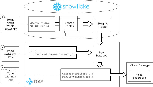
Step 1: Stage data in Snowflake#
When working with databases, it is best to take advantage of native join and aggregation features of the database prior to ingesting data into Ray Datasets. Ray datasets is designed to power machine learning workflows, and does not provide some typical analytics capabilities like large joins. For these reasons, as first step, the data required for training the model will be staged to a table within Snowflake prior to reading with the Ray Snowflake connector.
The code below creates a dataset of customer returns data from several Snowflake sample tables. We will use this data throughtout the train, tune and scoring process. In the code below, we use the Ray Snowflake connector to run DDL and DML, but you could just as easily use the Snowflake Python API. By using the Ray connector, the connection logic is unified in a single API.
Note: The data set size is set to be small to keep execution times small. If you would like to try larger dataset size, increase the
DATASET_SIZEand be sure to have a large enough cluster defined.
NOTE: This table may have already been been loaded to the customer_returns table in when setting up sample data previously.
SIZE = 1000000
SRC = 'SNOWFLAKE_SAMPLE_DATA.TPCDS_SF10TCL'
print(f'creating table CUSTOMER_RETURNS')
with connector:
    connector.query(f"""
            CREATE TABLE IF NOT EXISTS CUSTOMER_RETURNS as (
                WITH cstmrs as (
                        SELECT
                            c_customer_sk as c_customer_sk,
                            c_current_cdemo_sk as c_current_cdemo_sk
                        FROM {SRC}.customer LIMIT {SIZE}),

                    sales as (
                        SELECT
                            c_customer_sk,
                            COUNT(c_customer_sk) as n_sales
                        FROM cstmrs JOIN {SRC}.store_sales ON c_customer_sk = ss_customer_sk
                        GROUP BY c_customer_sk),

                    rtrns as (
                        SELECT
                            c_customer_sk,
                            COUNT(c_customer_sk) as n_returns
                        FROM cstmrs JOIN {SRC}.store_returns ON c_customer_sk = sr_customer_sk
                        GROUP BY c_customer_sk)

                SELECT
                    cstmrs.c_customer_sk as customer_sk,
                    ZEROIFNULL(n_sales) as n_sales,
                    ZEROIFNULL(n_returns) as n_returns,
                    IFF(n_sales is null or n_sales = 0 or n_returns is null, 0, n_returns/n_sales) as return_probability,
                    demos.*
                FROM cstmrs
                JOIN {SRC}.customer_demographics as demos ON cstmrs.c_current_cdemo_sk = demos.cd_demo_sk
                LEFT OUTER JOIN sales on cstmrs.c_customer_sk = sales.c_customer_sk
                LEFT OUTER JOIN rtrns on cstmrs.c_customer_sk = rtrns.c_customer_sk
            )
    """)
creating table CUSTOMER_RETURNS
Step 2: Read data into Ray#
Now that we have created the data, we can read it with the connector. Since our data was stroed in a different databse and schema, pass these new values to the connector create method.
with connector:
    ds = connector.read_table('CUSTOMER_RETURNS')

ds.limit(10).to_pandas()
0%| | 0/1 [00:00<?, ?it/s]
Read progress: 0%| | 0/1 [00:00<?, ?it/s]
Read progress: 100%|███████████████████████████████████████████████████████████████████████████████████████████████████████████████████████████████████████████████████| 1/1 [00:02<00:00, 2.40s/it]
Read progress: 100%|███████████████████████████████████████████████████████████████████████████████████████████████████████████████████████████████████████████████████| 1/1 [00:02<00:00, 2.40s/it]
| CUSTOMER_SK | N_SALES | N_RETURNS | RETURN_PROBABILITY | CD_DEMO_SK | CD_GENDER | CD_MARITAL_STATUS | CD_EDUCATION_STATUS | CD_PURCHASE_ESTIMATE | CD_CREDIT_RATING | CD_DEP_COUNT | CD_DEP_EMPLOYED_COUNT | CD_DEP_COLLEGE_COUNT | |
|---|---|---|---|---|---|---|---|---|---|---|---|---|---|
| 0 | 1650347 | 389 | 41 | 0.105398 | 187143 | M | S | 2 yr Degree | 7000 | Low Risk | 5 | 4 | 0 |
| 1 | 34455966 | 824 | 74 | 0.089806 | 187144 | F | S | 2 yr Degree | 7000 | Low Risk | 5 | 4 | 0 |
| 2 | 34435622 | 360 | 36 | 0.100000 | 187145 | M | D | 2 yr Degree | 7000 | Low Risk | 5 | 4 | 0 |
| 3 | 34491426 | 374 | 35 | 0.093583 | 187145 | M | D | 2 yr Degree | 7000 | Low Risk | 5 | 4 | 0 |
| 4 | 1779004 | 375 | 42 | 0.112000 | 187145 | M | D | 2 yr Degree | 7000 | Low Risk | 5 | 4 | 0 |
| 5 | 7447500 | 380 | 51 | 0.134211 | 187146 | F | D | 2 yr Degree | 7000 | Low Risk | 5 | 4 | 0 |
| 6 | 2446212 | 397 | 42 | 0.105793 | 187147 | M | W | 2 yr Degree | 7000 | Low Risk | 5 | 4 | 0 |
| 7 | 7396410 | 369 | 46 | 0.124661 | 187149 | M | U | 2 yr Degree | 7000 | Low Risk | 5 | 4 | 0 |
| 8 | 2411252 | 401 | 34 | 0.084788 | 187149 | M | U | 2 yr Degree | 7000 | Low Risk | 5 | 4 | 0 |
| 9 | 34540383 | 367 | 36 | 0.098093 | 187151 | M | M | 4 yr Degree | 7000 | Low Risk | 5 | 4 | 0 |
Step 3: Train#
Now that the data is read into a Ray dataset, we can use it to train or tune a LighGBM model.
Prepare the data
After reading the data, it is likely neccesary to do some simple manipualtions, like dropping columns splitting it into training and test sets.
DROP_COLUMNS = ['N_SALES', 'N_RETURNS', 'CD_DEMO_SK']

ds = ds.drop_columns(DROP_COLUMNS).repartition(100)
train_dataset, valid_dataset = ds.train_test_split(test_size=0.3)
0%| | 0/9 [00:00<?, ?it/s]
Read->Map_Batches: 0%| | 0/9 [00:00<?, ?it/s]
Read->Map_Batches: 11%|███████████████▉ | 1/9 [00:00<00:05, 1.42it/s]
Read->Map_Batches: 22%|███████████████████████████████▊ | 2/9 [00:01<00:04, 1.56it/s]
Read->Map_Batches: 33%|███████████████████████████████████████████████▋ | 3/9 [00:02<00:05, 1.04it/s]
Read->Map_Batches: 44%|███████████████████████████████████████████████████████████████▌ | 4/9 [00:02<00:03, 1.59it/s]
Read->Map_Batches: 67%|███████████████████████████████████████████████████████████████████████████████████████████████▎ | 6/9 [00:02<00:01, 2.81it/s]
Read->Map_Batches: 89%|███████████████████████████████████████████████████████████████████████████████████████████████████████████████████████████████ | 8/9 [00:03<00:00, 3.81it/s]
Read->Map_Batches: 100%|███████████████████████████████████████████████████████████████████████████████████████████████████████████████████████████████████████████████| 9/9 [00:03<00:00, 3.41it/s]
Read->Map_Batches: 100%|███████████████████████████████████████████████████████████████████████████████████████████████████████████████████████████████████████████████| 9/9 [00:03<00:00, 2.46it/s]
0%| | 0/100 [00:00<?, ?it/s]
Repartition: 0%| | 0/100 [00:00<?, ?it/s]
Repartition: 24%|██████████████████████████████████▊ | 24/100 [00:00<00:00, 219.17it/s]
Repartition: 46%|██████████████████████████████████████████████████████████████████▋ | 46/100 [00:00<00:00, 135.24it/s]
Repartition: 62%|██████████████████████████████████████████████████████████████████████████████████████████▌ | 62/100 [00:02<00:02, 17.05it/s]
Repartition: 71%|███████████████████████████████████████████████████████████████████████████████████████████████████████▋ | 71/100 [00:02<00:01, 20.69it/s]
Repartition: 82%|███████████████████████████████████████████████████████████████████████████████████████████████████████████████████████▋ | 82/100 [00:02<00:00, 26.87it/s]
Repartition: 91%|████████████████████████████████████████████████████████████████████████████████████████████████████████████████████████████████████▊ | 91/100 [00:02<00:00, 32.05it/s]
Repartition: 100%|█████████████████████████████████████████████████████████████████████████████████████████████████████████████████████████████████████████████████| 100/100 [00:03<00:00, 38.24it/s]
Repartition: 100%|█████████████████████████████████████████████████████████████████████████████████████████████████████████████████████████████████████████████████| 100/100 [00:03<00:00, 32.19it/s]
Create preprocessors
In Ray Air, all trainers, tuners and predcitors allow for the addition of preprocessors. Preprocessors help to featurize data, by providing common operations like on-hot-encoding, categorizing, scaling, etc. For more on the available preprocessors, read the RayAIR docs. The code below will use a chain of pre-processors. The BatchMapper will drop the ID column so it wont be used when training. The Categorizer will categorize columns, and the StandardScaler will scale columns. All of the pre-processing logic only modifes the data as it is being passed into training algorithms, and the underlying dataset will remain the same.
from ray.data.preprocessors import Chain, BatchMapper, Categorizer, StandardScaler

ID_COLUMN = 'CUSTOMER_SK'
CATEGORICAL_COLUMNS = ['CD_GENDER', 'CD_MARITAL_STATUS', 'CD_EDUCATION_STATUS', 'CD_CREDIT_RATING']
SCALAR_COLUMNS = ['CD_PURCHASE_ESTIMATE', 'CD_DEP_COUNT', 'CD_DEP_EMPLOYED_COUNT', 'CD_DEP_COLLEGE_COUNT']

# Scale some random columns, and categorify the categorical_column,
# allowing LightGBM to use its built-in categorical feature support
preprocessor = Chain(
    BatchMapper(lambda df: df.drop(ID_COLUMN, axis=1)),
    Categorizer(CATEGORICAL_COLUMNS),
    StandardScaler(columns=SCALAR_COLUMNS)
)
Configure scaling
Training requires compute infrastructure, and specifying what type is needed to optimize your training time and costs. When first beginning, it is best to start with a small dataset size and compute to get things working and then scale up data and compute together. Below we create a ScalingConfig that provides 10 workers for distributed trianing. This will likely keep training on a single instance. We also don’t request GPU’s.
from ray.air.config import ScalingConfig

scaling_config=ScalingConfig(num_workers=10, use_gpu=False),
Create a trainer
Now that we have everything required, we can create a trainer. In Ray AIR, the logic to create a trainer and fit it are very simliar. The main differences are in the parameters passed to the algorithm. This makes it easy to swap out algorithms. For example, swapping LightGBM for XGBoost, or even PyTorch tabular, will typically be just a few lines of code.
from ray.train.lightgbm import LightGBMTrainer

TARGET_COLUMN = 'RETURN_PROBABILITY'

# LightGBM specific params
params = {
    "objective": "regression",
    "metric": ["rmse", "mae"],
}

trainer = LightGBMTrainer(
    scaling_config=ScalingConfig(num_workers=2, use_gpu=False),
    label_column=TARGET_COLUMN,
    params=params,
    datasets={"train": train_dataset, "valid": valid_dataset},
    preprocessor=preprocessor,
    num_boost_round=10
)
Fit the model
Now that the trainer is defined, al that is required is to call fit to begin the training process. The fit method will return a results object that containes the model checkpoint as well as model training metrics.
result = trainer.fit()
Current time: 2022-11-20 13:10:18 (running for 00:00:27.22)
Memory usage on this node: 4.3/30.9 GiB
Using FIFO scheduling algorithm.
Resources requested: 0/52 CPUs, 0/0 GPUs, 0.0/140.4 GiB heap, 0.0/56.91 GiB objects
Result logdir: /home/ray/ray_results/LightGBMTrainer_2022-11-20_13-09-50
Number of trials: 1/1 (1 TERMINATED)
| Trial name | status | loc | iter | total time (s) | train-rmse | train-l1 | valid-rmse |
|---|---|---|---|---|---|---|---|
| LightGBMTrainer_abeb6_00000 | TERMINATED | 10.0.159.206:907 | 11 | 12.9436 | 0.0269048 | 0.0183024 | 0.0270086 |
(_RemoteRayLightGBMActor pid=1017, ip=10.0.159.206)
[LightGBM] [Info] Trying to bind port 55541...
(_RemoteRayLightGBMActor pid=1017, ip=10.0.159.206)
[LightGBM] [Info] Binding port 55541 succeeded
(_RemoteRayLightGBMActor pid=1017, ip=10.0.159.206)
[LightGBM] [Info] Listening...
(_RemoteRayLightGBMActor pid=1016, ip=10.0.159.206)
[LightGBM] [Info] Trying to bind port 48245...
(_RemoteRayLightGBMActor pid=1016, ip=10.0.159.206)
[LightGBM] [Info] Binding port 48245 succeeded
(_RemoteRayLightGBMActor pid=1016, ip=10.0.159.206)
[LightGBM] [Info] Listening...
(_RemoteRayLightGBMActor pid=1016, ip=10.0.159.206)
[LightGBM] [Warning] Connecting to rank 1 failed, waiting for 200 milliseconds
(_RemoteRayLightGBMActor pid=1017, ip=10.0.159.206)
[LightGBM] [Info] Connected to rank 0
(_RemoteRayLightGBMActor pid=1017, ip=10.0.159.206)
[LightGBM] [Info] Local rank: 1, total number of machines: 2
(_RemoteRayLightGBMActor pid=1016, ip=10.0.159.206)
[LightGBM] [Info] Connected to rank 1
(_RemoteRayLightGBMActor pid=1016, ip=10.0.159.206)
[LightGBM] [Info] Local rank: 0, total number of machines: 2
(_RemoteRayLightGBMActor pid=1017, ip=10.0.159.206)
[LightGBM] [Warning] num_threads is set=2, n_jobs=-1 will be ignored. Current value: num_threads=2
(_RemoteRayLightGBMActor pid=1016, ip=10.0.159.206)
[LightGBM] [Warning] num_threads is set=2, n_jobs=-1 will be ignored. Current value: num_threads=2
Result for LightGBMTrainer_abeb6_00000:
  date: 2022-11-20_13-10-08
  done: false
  experiment_id: 3d58679910414275af48e518881f5a02
  hostname: ip-10-0-159-206
  iterations_since_restore: 1
  node_ip: 10.0.159.206
  pid: 907
  time_since_restore: 12.153637409210205
  time_this_iter_s: 12.153637409210205
  time_total_s: 12.153637409210205
  timestamp: 1668978608
  timesteps_since_restore: 0
  train-l1: 0.01830608920339265
  train-rmse: 0.026910509092779773
  training_iteration: 1
  trial_id: abeb6_00000
  valid-l1: 0.01836421957812595
  valid-rmse: 0.027008004632721412
  warmup_time: 0.016459941864013672
Result for LightGBMTrainer_abeb6_00000:
  date: 2022-11-20_13-10-09
  done: true
  experiment_id: 3d58679910414275af48e518881f5a02
  experiment_tag: '0'
  hostname: ip-10-0-159-206
  iterations_since_restore: 11
  node_ip: 10.0.159.206
  pid: 907
  time_since_restore: 12.943555355072021
  time_this_iter_s: 0.38719749450683594
  time_total_s: 12.943555355072021
  timestamp: 1668978609
  timesteps_since_restore: 0
  train-l1: 0.01830242573779587
  train-rmse: 0.026904803701133656
  training_iteration: 11
  trial_id: abeb6_00000
  valid-l1: 0.018364583890927544
  valid-rmse: 0.02700859654265805
  warmup_time: 0.016459941864013672
Score a model#
Once there is a trained model, we can use it to score data. The flow for training and scoring are similar in that data is staged in Snowflake and read into a Ray dataset with the connector. Once the data is read in, the previously created model checkpoint can be used to creat a batch predictor for scoring. Scored data can then be written back into Snowflake with the connector.
The typical logical flow for a batch scoring in Snowflake with Ray AIR is the following:
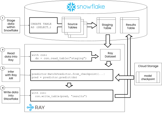
Steps 1-2: Stage and read data#
Since the data has already been staged and loaded, we dont need any extra code to do that now. Typically, you will have a script for training, and a script for scoring that will be run independently. THe staging and loading of data should be sperated into a shared script that can be used by each of these workflows.
Step 3: Score the data#
The previously trained checkpoint can be used to create a predictor. This predictor will already contain the pre-processors used to train the model. All that is needed is to drop the target column before feeding it into the model to simulate a real dataset where we dont know the results.
Note: Typically model checkpoints will be stored in a model registry provided by Weights and Biases or MLFlow, or into an objects store like S3. Checkpoints are written and read using the checkpoint API.
from ray.train.batch_predictor import BatchPredictor
from ray.train.lightgbm import LightGBMPredictor

predictor = BatchPredictor.from_checkpoint(
    result.checkpoint, LightGBMPredictor
)

test_dataset = valid_dataset.drop_columns(TARGET_COLUMN)
predictions = predictor.predict(test_dataset, keep_columns=[ID_COLUMN])
predictions.limit(10).to_pandas()
0%| | 0/30 [00:00<?, ?it/s]
Map_Batches: 0%| | 0/30 [00:00<?, ?it/s]
Map_Batches: 3%|████▉ | 1/30 [00:00<00:04, 6.61it/s]
Map_Batches: 10%|██████████████▊ | 3/30 [00:02<00:21, 1.25it/s]
Map_Batches: 20%|█████████████████████████████▌ | 6/30 [00:02<00:09, 2.51it/s]
Map_Batches: 27%|███████████████████████████████████████▍ | 8/30 [00:02<00:06, 3.44it/s]
Map_Batches: 47%|████████████████████████████████████████████████████████████████████▌ | 14/30 [00:02<00:02, 7.85it/s]
Map_Batches: 53%|██████████████████████████████████████████████████████████████████████████████▍ | 16/30 [00:03<00:01, 8.48it/s]
Map_Batches: 73%|███████████████████████████████████████████████████████████████████████████████████████████████████████████▊ | 22/30 [00:03<00:00, 14.18it/s]
Map_Batches: 83%|██████████████████████████████████████████████████████████████████████████████████████████████████████████████████████████▌ | 25/30 [00:03<00:00, 15.87it/s]
Map_Batches: 100%|███████████████████████████████████████████████████████████████████████████████████████████████████████████████████████████████████████████████████| 30/30 [00:03<00:00, 20.90it/s]
Map_Batches: 100%|███████████████████████████████████████████████████████████████████████████████████████████████████████████████████████████████████████████████████| 30/30 [00:03<00:00, 8.47it/s]
0%| | 0/30 [00:00<?, ?it/s]
Map_Batches: 0%| | 0/30 [00:00<?, ?it/s]
Map Progress (1 actors 0 pending): 0%| | 0/30 [00:03<?, ?it/s]
Map Progress (1 actors 1 pending): 0%| | 0/30 [00:03<?, ?it/s]
Map Progress (1 actors 1 pending): 3%|████▏ | 1/30 [00:03<01:52, 3.89s/it]
Map Progress (1 actors 1 pending): 10%|████████████▌ | 3/30 [00:04<00:28, 1.05s/it]
Map Progress (1 actors 1 pending): 17%|█████████████████████ | 5/30 [00:04<00:13, 1.83it/s]
Map Progress (1 actors 1 pending): 23%|█████████████████████████████▍ | 7/30 [00:04<00:07, 2.94it/s]
Map Progress (1 actors 1 pending): 30%|█████████████████████████████████████▊ | 9/30 [00:04<00:04, 4.25it/s]
Map Progress (1 actors 1 pending): 37%|█████████████████████████████████████████████▊ | 11/30 [00:04<00:03, 5.73it/s]
Map Progress (1 actors 1 pending): 43%|██████████████████████████████████████████████████████▏ | 13/30 [00:04<00:02, 7.30it/s]
Map Progress (1 actors 1 pending): 50%|██████████████████████████████████████████████████████████████▌ | 15/30 [00:04<00:01, 8.86it/s]
Map Progress (1 actors 1 pending): 57%|██████████████████████████████████████████████████████████████████████▊ | 17/30 [00:04<00:01, 10.44it/s]
Map Progress (1 actors 1 pending): 63%|███████████████████████████████████████████████████████████████████████████████▏ | 19/30 [00:04<00:00, 11.75it/s]
Map Progress (1 actors 1 pending): 70%|███████████████████████████████████████████████████████████████████████████████████████▌ | 21/30 [00:05<00:00, 12.91it/s]
Map Progress (1 actors 1 pending): 77%|███████████████████████████████████████████████████████████████████████████████████████████████▊ | 23/30 [00:05<00:00, 13.75it/s]
Map Progress (1 actors 1 pending): 83%|████████████████████████████████████████████████████████████████████████████████████████████████████████▏ | 25/30 [00:05<00:00, 14.37it/s]
Map Progress (1 actors 1 pending): 90%|████████████████████████████████████████████████████████████████████████████████████████████████████████████████▌ | 27/30 [00:05<00:00, 14.81it/s]
Map Progress (1 actors 1 pending): 97%|████████████████████████████████████████████████████████████████████████████████████████████████████████████████████████▊ | 29/30 [00:05<00:00, 15.23it/s]
Map Progress (1 actors 1 pending): 100%|█████████████████████████████████████████████████████████████████████████████████████████████████████████████████████████████| 30/30 [00:05<00:00, 5.28it/s]
| predictions | CUSTOMER_SK | |
|---|---|---|
| 0 | 0.102189 | 1639066 |
| 1 | 0.102189 | 34453320 |
| 2 | 0.102316 | 7465318 |
| 3 | 0.102375 | 50443610 |
| 4 | 0.102375 | 2535927 |
| 5 | 0.102375 | 1663533 |
| 6 | 0.102375 | 7505486 |
| 7 | 0.102375 | 7398215 |
| 8 | 0.102375 | 2570281 |
| 9 | 0.102320 | 1725142 |
Step 4: Write data to Snowflake#
Now that we have the predictions we can write them into a SNowflake table.
import os
userid = os.getenv('ANYSCALE_EXPERIMENTAL_USERNAME')
table = 'CUSTOMER_PREDICTIONS_'+userid.upper()

# create a table
print('creating table '+table)
with connector:
    connector.query(f'''
        CREATE OR REPLACE TABLE {table} (
            PREDICTIONS FLOAT NOT NULL,
            CUSTOMER_SK VARCHAR(20) NOT NULL
	    )
    ''')

# write to the table
with connector:
    connector.write_table(predictions, table)

with connector:
    ds2 = connector.read_table(table)

ds2.limit(10).to_pandas()
creating table CUSTOMER_PREDICTIONS_ERIC_GREENE_A9C7590
0%| | 0/30 [00:00<?, ?it/s]
Write Progress: 0%| | 0/30 [00:00<?, ?it/s]
Write Progress: 3%|████▊ | 1/30 [00:00<00:23, 1.25it/s]
Write Progress: 7%|█████████▋ | 2/30 [00:01<00:12, 2.21it/s]
Write Progress: 23%|█████████████████████████████████▊ | 7/30 [00:01<00:02, 8.62it/s]
Write Progress: 33%|████████████████████████████████████████████████ | 10/30 [00:01<00:01, 12.09it/s]
Write Progress: 47%|███████████████████████████████████████████████████████████████████▏ | 14/30 [00:01<00:00, 16.22it/s]
Write Progress: 60%|██████████████████████████████████████████████████████████████████████████████████████▍ | 18/30 [00:01<00:00, 18.71it/s]
Write Progress: 70%|████████████████████████████████████████████████████████████████████████████████████████████████████▊ | 21/30 [00:03<00:01, 5.58it/s]
Write Progress: 77%|██████████████████████████████████████████████████████████████████████████████████████████████████████████████▍ | 23/30 [00:03<00:01, 6.48it/s]
Write Progress: 97%|███████████████████████████████████████████████████████████████████████████████████████████████████████████████████████████████████████████▏ | 29/30 [00:03<00:00, 10.86it/s]
Write Progress: 100%|████████████████████████████████████████████████████████████████████████████████████████████████████████████████████████████████████████████████| 30/30 [00:04<00:00, 6.07it/s]
0%| | 0/1 [00:00<?, ?it/s]
Read progress: 0%| | 0/1 [00:00<?, ?it/s]
Read progress: 100%|██████████████████████████████████████████████████████████████████████████████████████████████████████████████████████████████████████████████████| 1/1 [00:00<00:00, 870.19it/s]
| PREDICTIONS | CUSTOMER_SK | |
|---|---|---|
| 0 | 0.102312 | 7496063 |
| 1 | 0.102312 | 7562373 |
| 2 | 0.102331 | 7532594 |
| 3 | 0.102384 | 7436509 |
| 4 | 0.102313 | 7555153 |
| 5 | 0.102235 | 7576147 |
| 6 | 0.102236 | 34472610 |
| 7 | 0.102311 | 7559201 |
| 8 | 0.102312 | 34549247 |
| 9 | 0.102312 | 1829286 |